3.加权基因共表达网络分析（WGCNA）

#======================================
# 原创代码无删减，编写不易，论文使用本代码绘图，请引用：www.tcmbiohub.com

# 祝大家投稿顺利！

## ========================================
#if (!requireNamespace("BiocManager", quietly = TRUE))
#    install.packages("BiocManager")
#BiocManager::install(c("GO.db", "preprocessCore", "impute", "limma"))

#install.packages(c("matrixStats", "Hmisc", "foreach", "doParallel", "fastcluster", "dynamicTreeCut", "survival")) 
#install.packages("WGCNA")


#加载包
library(limma)
library(WGCNA)

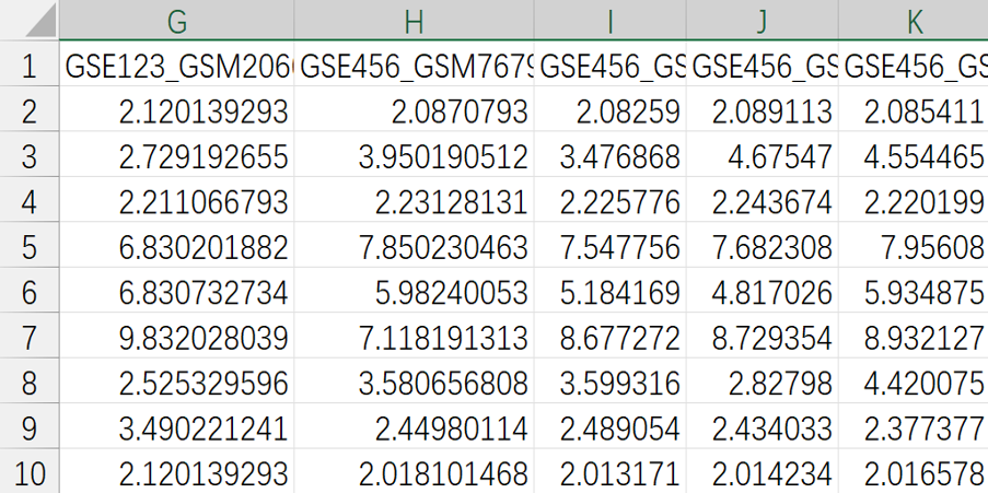
expFile="merge.normalize.txt"      #输入表达矩阵文件
diseaseName="Disease"                #热图展示的疾病分组名称
setwd("C:/Users/Administrator/Desktop/5.WGCNA")     #设置工作目录

#读取输入文件，对表达矩阵进行处理
rt=read.table(expFile, header=T, sep="\t", check.names=F)
rt=as.matrix(rt)
rownames(rt)=rt[,1]
exp=rt[,2:ncol(rt)]
dimnames=list(rownames(exp),colnames(exp))
data=matrix(as.numeric(as.matrix(exp)),nrow=nrow(exp),dimnames=dimnames)
data=avereps(data)
data=data[apply(data,1,sd)>0.5,]     #去除标准差小的基因

#获取样本的分组信息（用于后续绘图）
Type=gsub("(.*)\\_(.*)\\_(.*)", "\\3", colnames(data))
data=data[,order(Type)]
Type=gsub("(.*)\\_(.*)\\_(.*)", "\\3", colnames(data))
conCount=length(Type[Type=="Control"])
treatCount=length(Type[Type=="Treat"])
datExpr0=t(data)

###筛选缺失值
gsg = goodSamplesGenes(datExpr0, verbose = 3)
if (!gsg$allOK)
{
  # Optionally, print the gene and sample names that were removed:
  if (sum(!gsg$goodGenes)>0)
    printFlush(paste("Removing genes:", paste(names(datExpr0)[!gsg$goodGenes], collapse = ", ")))
  if (sum(!gsg$goodSamples)>0)
    printFlush(paste("Removing samples:", paste(rownames(datExpr0)[!gsg$goodSamples], collapse = ", ")))
  # Remove the offending genes and samples from the data:
  datExpr0 = datExpr0[gsg$goodSamples, gsg$goodGenes]
}

###样本聚类
sampleTree = hclust(dist(datExpr0), method = "average")
pdf(file = "1_sample_cluster.pdf", width = 9, height = 6)
par(cex = 0.6)
par(mar = c(0,4,2,0))
plot(sampleTree, main = "Sample clustering to detect outliers", sub="", xlab="", cex.lab = 1.5, cex.axis = 1.5, cex.main = 2)
###剪切阈值
abline(h = 20000, col = "red")
dev.off()

###剔除离群样本
clust = cutreeStatic(sampleTree, cutHeight=20000, minSize=10)
table(clust)
keepSamples = (clust==1)
datExpr0 = datExpr0[keepSamples, ]


###准备样本的分组信息
traitData=data.frame(Control=c(rep(1,conCount),rep(0,treatCount)),
                     Treat=c(rep(0,conCount),rep(1,treatCount)))
colnames(traitData)=c("Control", diseaseName)
row.names(traitData)=colnames(data)
fpkmSamples = rownames(datExpr0)
traitSamples =rownames(traitData)
sameSample=intersect(fpkmSamples,traitSamples)
datExpr0=datExpr0[sameSample,]
datTraits=traitData[sameSample,]


###再次进行样本聚类，得到样本聚类热图
sampleTree2 = hclust(dist(datExpr0), method = "average")
traitColors = numbers2colors(datTraits, signed = FALSE)
pdf(file="2_sample_heatmap.pdf", width=9, height=7)
plotDendroAndColors(sampleTree2, traitColors,
                    groupLabels = names(datTraits),
                    main = "Sample dendrogram and trait heatmap")
dev.off()

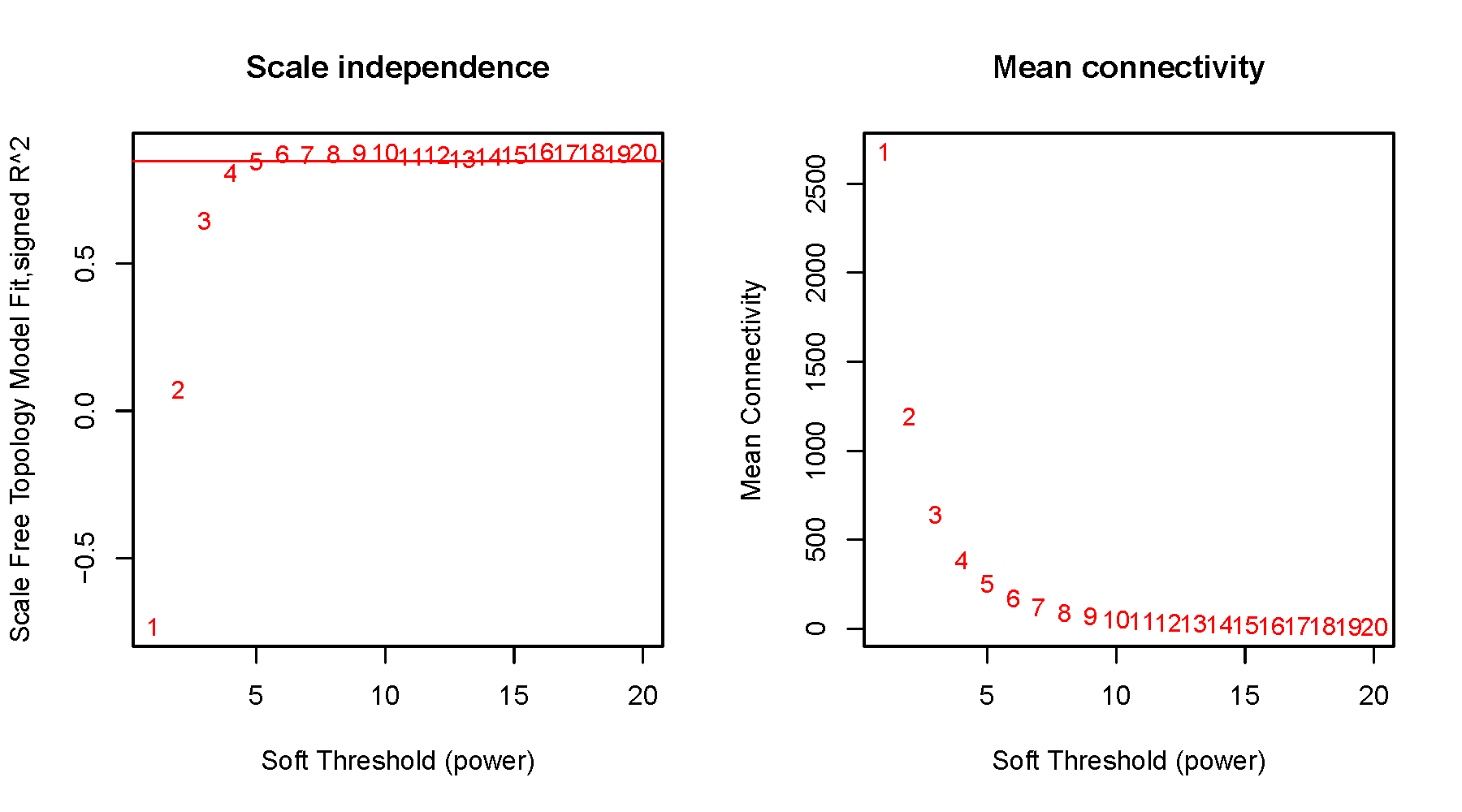
###power值筛选图
enableWGCNAThreads()   #开启多线程
powers = c(1:20)       #设置power值范围1:20
sft = pickSoftThreshold(datExpr0, powerVector = powers, verbose = 5)
pdf(file="3_scale_independence.pdf", width=9, height=5)
par(mfrow = c(1,2))
cex1 = 0.9
###无标度网络power值分布图
plot(sft$fitIndices[,1], -sign(sft$fitIndices[,3])*sft$fitIndices[,2],
     xlab="Soft Threshold (power)",ylab="Scale Free Topology Model Fit,signed R^2",type="n",
     main = paste("Scale independence"));
text(sft$fitIndices[,1], -sign(sft$fitIndices[,3])*sft$fitIndices[,2],
     labels=powers,cex=cex1,col="red");
abline(h=0.85, col="red") #阈值可修改
###平均连通性power值分布图
plot(sft$fitIndices[,1], sft$fitIndices[,5],
     xlab="Soft Threshold (power)",ylab="Mean Connectivity", type="n",
     main = paste("Mean connectivity"))
text(sft$fitIndices[,1], sft$fitIndices[,5], labels=powers, cex=cex1,col="red")
dev.off()

###邻接矩阵转换
sft      #查看最优power值
softPower =sft$powerEstimate      #最优power值
adjacency = adjacency(datExpr0, power = softPower)
softPower

###TOM相似性计算
TOM = TOMsimilarity(adjacency)
dissTOM = 1-TOM

###基因聚类
geneTree = hclust(as.dist(dissTOM), method = "average");
pdf(file="4_gene_clustering.pdf", width=8, height=6)
plot(geneTree, xlab="", sub="", main = "Gene clustering on TOM-based dissimilarity",
     labels = FALSE, hang = 0.04)
dev.off()


###动态树切割识别模块（得到每个模块对应的基因）
minModuleSize = 60      #模块最小基因数（每个模块至少60个基因）
dynamicMods = cutreeDynamic(dendro = geneTree, distM = dissTOM,
                            deepSplit = 2, pamRespectsDendro = FALSE,
                            minClusterSize = minModuleSize);
table(dynamicMods)
dynamicColors = labels2colors(dynamicMods)
table(dynamicColors)
pdf(file="5_Dynamic_Tree.pdf", width=8, height=6)
plotDendroAndColors(geneTree, dynamicColors, "Dynamic Tree Cut",
                    dendroLabels = FALSE, hang = 0.03,
                    addGuide = TRUE, guideHang = 0.05,
                    main = "Gene dendrogram and module colors")
dev.off()


###对模块进行聚类，找出相似模块
MEList = moduleEigengenes(datExpr0, colors = dynamicColors)
MEs = MEList$eigengenes
MEDiss = 1-cor(MEs);
METree = hclust(as.dist(MEDiss), method = "average")
pdf(file="6_Clustering_module.pdf", width=7, height=6)
plot(METree, main = "Clustering of module eigengenes",
     xlab = "", sub = "")
MEDissThres = 0.25     #剪切高度可修改
abline(h=MEDissThres, col = "red")
dev.off()


###相似模块合并（得到最终的共表达模块）
merge = mergeCloseModules(datExpr0, dynamicColors, cutHeight = MEDissThres, verbose = 3)
mergedColors = merge$colors
mergedMEs = merge$newMEs
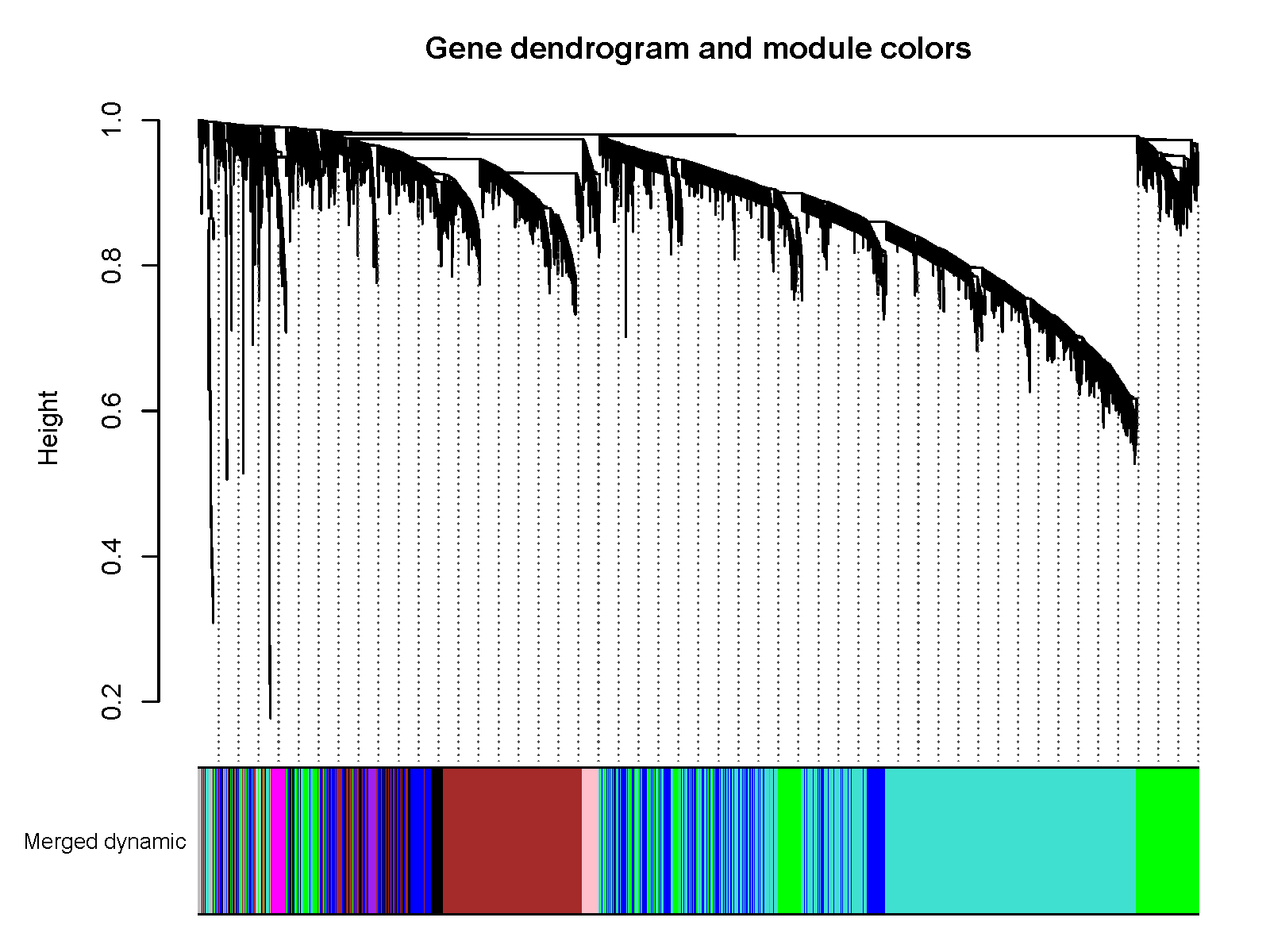
pdf(file="7_merged_dynamic.pdf", width=8, height=6)
plotDendroAndColors(geneTree, mergedColors, "Merged dynamic",
                    dendroLabels = FALSE, hang = 0.03,
                    addGuide = TRUE, guideHang = 0.05,
                    main = "Gene dendrogram and module colors")
dev.off()
moduleColors = mergedColors
table(moduleColors)
colorOrder = c("grey", standardColors(50))
moduleLabels = match(moduleColors, colorOrder)-1
MEs = mergedMEs


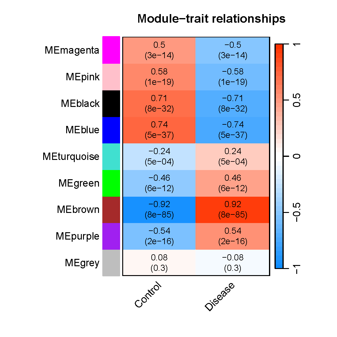
###模块与性状相关性热图绘制
nGenes = ncol(datExpr0)
nSamples = nrow(datExpr0)
moduleTraitCor = cor(MEs, datTraits, use = "p")
moduleTraitPvalue = corPvalueStudent(moduleTraitCor, nSamples)
pdf(file="8_Module_trait.pdf", width=5.5, height=5.5)
textMatrix = paste(signif(moduleTraitCor, 2), "\n(",
                   signif(moduleTraitPvalue, 1), ")", sep = "")
dim(textMatrix) = dim(moduleTraitCor)
par(mar = c(5, 10, 3, 3))
labeledHeatmap(Matrix = moduleTraitCor,
               xLabels = names(datTraits),    #X轴标签
               yLabels = names(MEs),          #Y轴标签
               ySymbols = names(MEs),
               colorLabels = FALSE,
               colors = blueWhiteRed(50),    #热图颜色
               textMatrix = textMatrix,      #热图展示文字信息
               setStdMargins = FALSE,
               cex.text = 0.85,          #文字大小
               zlim = c(-1,1),           #相关系数范围
               main = paste("Module-trait relationships"))     #热图标题
dev.off()

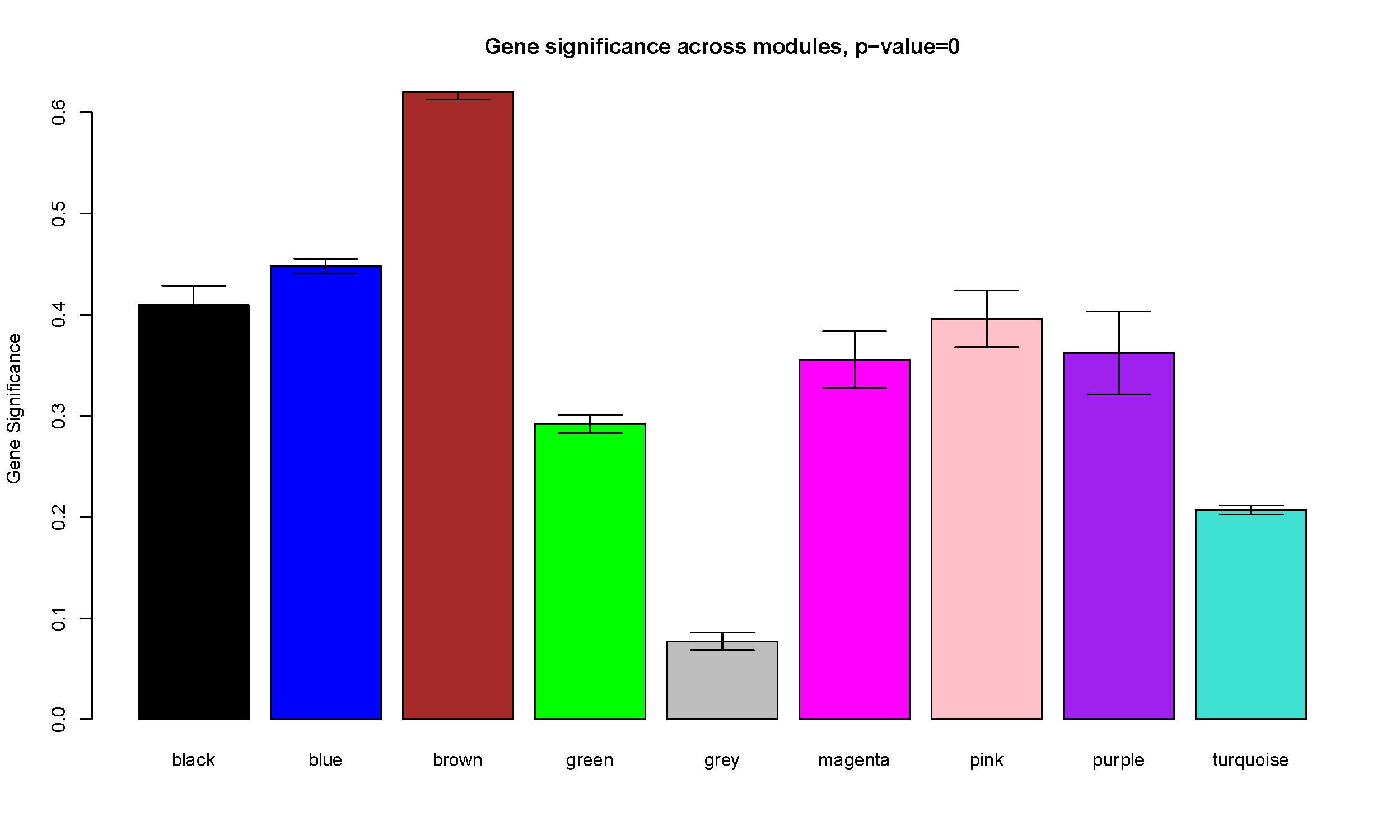
###模块重要性柱状图
y=datTraits[,1]
GS1=as.numeric(cor(y, datExpr0, use="p"))
GeneSignificance=abs(GS1)
ModuleSignificance=tapply(GeneSignificance, mergedColors, mean, na.rm=T)
pdf(file="9_GeneSignificance.pdf", width=12.5, height=7.5)
plotModuleSignificance(GeneSignificance, mergedColors)
dev.off()

###输出每个模块的基因列表
for (mod in 1:nrow(table(moduleColors))){  
	modules = names(table(moduleColors))[mod]
	probes = colnames(datExpr0)
	inModule = (moduleColors == modules)
	modGenes = probes[inModule]
	write.table(modGenes, file =paste0("module_",modules,".txt"),sep="\t",row.names=F,col.names=F,quote=F)
}

#======================================
# 原创代码无删减，编写不易，若投稿使用代码绘图，请引用：www.tcmbiohub.com

# 祝大家投稿顺利！