#======================================
# 原创代码无删减,编写不易,若使用代码绘图,请引用:www.tcmbiohub.com
# 祝大家投稿顺利!
## =========================================================
.libPaths(c(Sys.getenv("R_LIBS_USER"), .libPaths()))
rm(list = ls())
## 1) Packages ----
pkgs <- c("ggplot2","ggridges","dplyr","tidyr","readr","stringr","forcats","viridis","purrr","patchwork")
to_install <- pkgs[!pkgs %in% rownames(installed.packages())]
if (length(to_install) > 0) install.packages(to_install, dependencies = TRUE)
invisible(lapply(pkgs, library, character.only = TRUE))
## 2) File paths ----
up_file <- "uptop20.txt"
down_file <- "downtop20.txt"
if (!file.exists(up_file)) stop("Cannot find file: ", up_file)
if (!file.exists(down_file)) stop("Cannot find file: ", down_file)
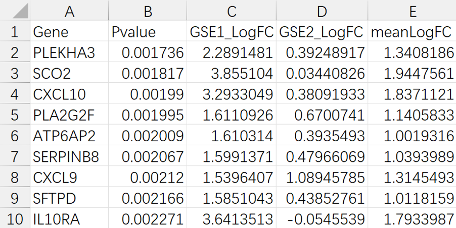
## 3) Read data ----
up <- readr::read_tsv(up_file, show_col_types = FALSE)
down <- readr::read_tsv(down_file, show_col_types = FALSE)
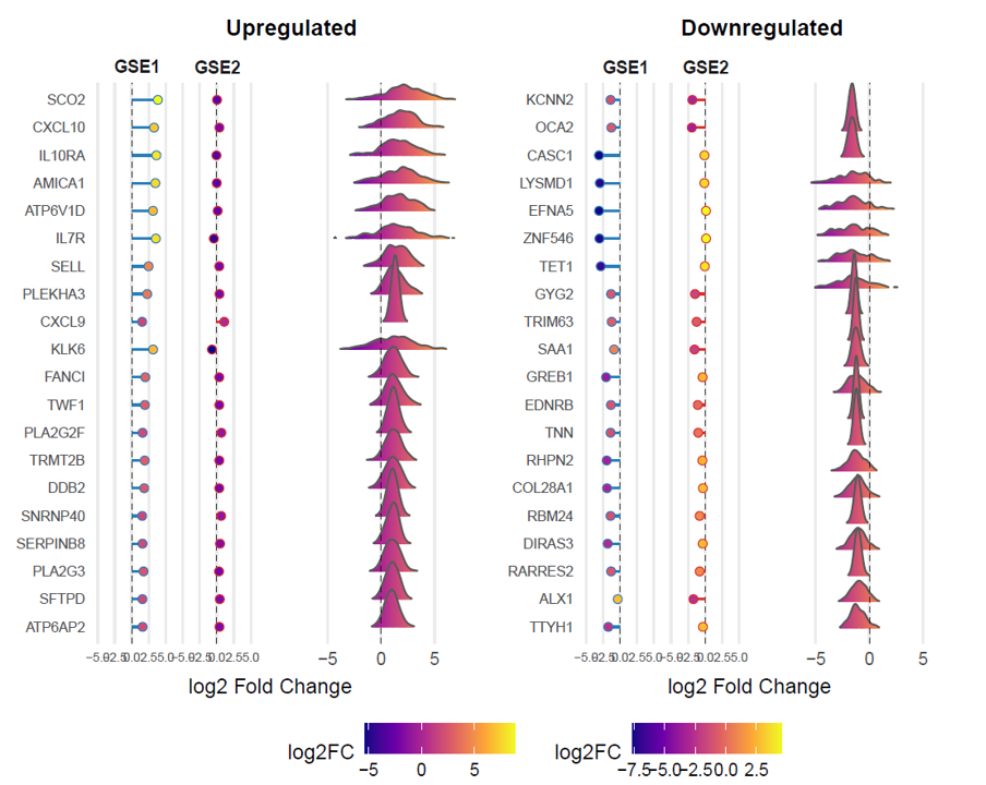
up$Group <- "Upregulated"
down$Group <- "Downregulated"
df <- dplyr::bind_rows(up, down)
## 4) Check required columns ----
required_cols <- c("Gene", "meanLogFC", "GSE1_LogFC", "GSE2_LogFC")
missing_cols <- setdiff(required_cols, colnames(df))
if (length(missing_cols) > 0) stop("Missing required column(s): ", paste(missing_cols, collapse = ", "))
df <- df %>%
mutate(
Group = factor(Group, levels = c("Upregulated","Downregulated")),
Gene = as.character(Gene),
meanLogFC = as.numeric(meanLogFC),
GSE1_LogFC = as.numeric(GSE1_LogFC),
GSE2_LogFC = as.numeric(GSE2_LogFC)
)
## 5) Order genes within each group ----
df_up <- df %>% filter(Group == "Upregulated") %>% arrange(desc(meanLogFC))
df_dn <- df %>% filter(Group == "Downregulated") %>% arrange(meanLogFC)
## 6) Estimate ridge width (sd) ----
df <- df %>%
rowwise() %>%
mutate(sd_est = max(0.15, abs(GSE1_LogFC - GSE2_LogFC) / 2)) %>%
ungroup()
## 7) Simulate per-gene distributions for ridges ----
set.seed(123)
n_per_gene <- 250
sim_df <- df %>%
select(Gene, Group, meanLogFC, sd_est) %>%
mutate(sim = purrr::map2(meanLogFC, sd_est, ~ rnorm(n_per_gene, mean = .x, sd = .y))) %>%
tidyr::unnest(sim) %>%
rename(simLogFC = sim)
## 8) Build separate datasets (each panel keeps its own gene order) ----
sim_up <- sim_df %>%
filter(Group == "Upregulated") %>%
mutate(Gene = factor(Gene, levels = df_up$Gene)) %>%
mutate(Gene = forcats::fct_rev(Gene))
sim_dn <- sim_df %>%
filter(Group == "Downregulated") %>%
mutate(Gene = factor(Gene, levels = df_dn$Gene)) %>%
mutate(Gene = forcats::fct_rev(Gene))
## 9) Unify x-axis range for ridge panels ----
x_lim <- max(abs(df$meanLogFC) + 3 * df$sd_est, na.rm = TRUE)
x_lim <- ceiling(x_lim * 1.05)
## 10) Prepare annotation (2 cohort columns) ----
## Choose style: "lollipop" (dot+segment), "dot", or "bar"
anno_style <- "lollipop"
prep_anno <- function(df_group, gene_levels) {
anno <- df_group %>%
select(Gene, GSE1_LogFC, GSE2_LogFC) %>%
tidyr::pivot_longer(
cols = c(GSE1_LogFC, GSE2_LogFC),
names_to = "Cohort",
values_to = "logFC"
) %>%
mutate(
Cohort = recode(Cohort,
GSE1_LogFC = "GSE1",
GSE2_LogFC = "GSE2"),
Cohort = factor(Cohort, levels = c("GSE1", "GSE2")),
Gene = factor(Gene, levels = gene_levels),
Gene = forcats::fct_rev(Gene)
)
anno
}
anno_up <- prep_anno(df_up, df_up$Gene)
anno_dn <- prep_anno(df_dn, df_dn$Gene)
## annotation xlim (global, shared)
anno_xlim <- max(abs(c(df$GSE1_LogFC, df$GSE2_LogFC)), na.rm = TRUE)
anno_xlim <- ceiling(anno_xlim * 1.05)
## 11) Annotation plot function (COHORT-colored segments + gradient filled dots) ----
make_anno <- function(anno_dat) {
# Keep this FALSE to avoid duplicate log2FC legends (ridge already has one)
show_anno_legend <- FALSE
p <- ggplot(anno_dat, aes(y = Gene)) +
geom_vline(xintercept = 0, linetype = "dashed", linewidth = 0.35, alpha = 0.8)
if (anno_style == "bar") {
p <- p +
geom_col(aes(x = logFC, fill = logFC, color = Cohort),
width = 0.68, linewidth = 0.25)
} else if (anno_style == "dot") {
p <- p +
geom_point(aes(x = logFC, fill = logFC, color = Cohort),
shape = 21, size = 2.1, stroke = 0.45)
} else { # lollipop
p <- p +
geom_segment(aes(x = 0, xend = logFC, yend = Gene, color = Cohort),
linewidth = 0.55, alpha = 0.95) +
geom_point(aes(x = logFC, fill = logFC, color = Cohort),
shape = 21, size = 2.1, stroke = 0.45)
}
p <- p +
facet_grid(. ~ Cohort) +
coord_cartesian(xlim = c(-anno_xlim, anno_xlim)) +
scale_fill_viridis_c(option = "plasma", name = "log2FC") +
scale_color_manual(
values = c("GSE1" = "#1F77B4", "GSE2" = "#D62728"),
name = NULL
) +
labs(x = NULL, y = NULL) +
theme_minimal(base_size = 12) +
theme(
panel.grid.major.y = element_blank(),
panel.grid.minor = element_blank(),
axis.text.y = element_text(size = 8),
axis.text.x = element_text(size = 7),
axis.ticks.x = element_blank(),
strip.text = element_text(size = 10, face = "bold"),
legend.position = "bottom",
plot.margin = margin(t = 6, r = 6, b = 6, l = 6)
)
if (!show_anno_legend) {
p <- p + guides(fill = "none", color = "none")
}
p
}
p_anno_up <- make_anno(anno_up)
p_anno_dn <- make_anno(anno_dn)
## 12) Ridge plot function (hide y labels; annotation panel shows gene names) ----
make_ridge <- function(dat, panel_title) {
ggplot(dat, aes(x = simLogFC, y = Gene, fill = after_stat(x))) +
geom_density_ridges_gradient(
scale = 2.4,
rel_min_height = 0.01,
size = 0.25,
color = "grey35"
) +
geom_vline(xintercept = 0, linetype = "dashed", linewidth = 0.35, alpha = 0.8) +
coord_cartesian(xlim = c(-x_lim, x_lim)) +
scale_fill_viridis_c(option = "plasma", name = "log2FC") +
labs(
title = panel_title,
x = "log2 Fold Change (simulated around meanLogFC; width reflects between-cohort difference)",
y = NULL
) +
theme_minimal(base_size = 12) +
theme(
panel.grid.major.y = element_blank(),
panel.grid.minor = element_blank(),
axis.text.y = element_blank(),
axis.ticks.y = element_blank(),
plot.title = element_text(face = "bold", size = 13),
legend.position = "bottom",
plot.margin = margin(t = 6, r = 6, b = 6, l = 6)
)
}
p_ridge_up <- make_ridge(sim_up, "Upregulated (Top genes)")
p_ridge_dn <- make_ridge(sim_dn, "Downregulated (Top genes)")
## 13) Combine (annotation columns + ridge) for each group ----
p_up <- (p_anno_up + p_ridge_up) + patchwork::plot_layout(widths = c(0.43, 0.57))
p_dn <- (p_anno_dn + p_ridge_dn) + patchwork::plot_layout(widths = c(0.43, 0.57))
## 14) Combine Up/Down side-by-side and collect legend ----
p_all <- (p_up | p_dn) +
patchwork::plot_layout(guides = "collect") &
theme(legend.position = "bottom")
## 15) Save ----
out_pdf <- "Top20_RidgeHeatmap_with2Cohorts_DotBar_Colored.pdf"
ggsave(out_pdf, plot = p_all, width = 8, height = 6.5, units = "in", dpi = 300)
message("Done. Output saved: ", out_pdf)
#======================================
# 原创代码无删减,编写不易,若使用代码绘图,请引用:www.tcmbiohub.com
# 祝大家投稿顺利!
 TCM Bio Hub⠀⠀⠀